Sampling states from the SEI-SLR algorithm

The example runs the SEI-SLR algorithm to generate states uniformly distributed on the selection event.

import PSILOGIT
import numpy as np
from PSILOGIT.tools import *
from sklearn.linear_model import LogisticRegression, LogisticRegressionCV
import matplotlib.pyplot as plt

We build a model with a randomly generated dataset.

n = 10
p = 15
theta = np.zeros(p)
lamb = 2
model = PSILOGIT.PSILOGIT(truetheta=theta, regularization=lamb,  n=n, p=p)

We run the SEI-SLR algorithm.

def linear_temperature(t):
    return 0.2/np.log(t+1)
states, ls_FNR, energies = model.SEI_SLR(total_length_SEISLR_path=100000, backup_start_time=2000, temperature=linear_temperature, repulsing_force=True, random_start=True, conditioning_signs=False, seed=0)

0%|          | 0/100000 [00:00<?, ?it/s]

The size of the observed vector is small enough to compute exactly the states belonging to the selection event via an exhaustive search.

nbM_admissibles, ls_states_admissibles = model.compute_selection_event(compare_with_energy=True)
print('Size of the selection event: ', len(ls_states_admissibles))

Size of the selection event:  22

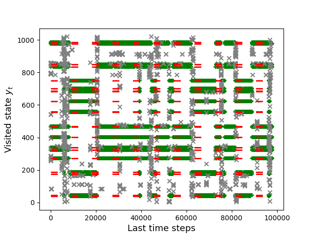
By running over the~$2^{10}$ possible vectors \(Y \in \{ 0,1\}^N\), we have previously computed exactly the selection event. In the following, we identify each vector \(Y \in \{0, 1\}^N\) with the number between~$0$ and~$2^N-1=1024$ that it represents in the base-2 numeral system. The following figure shows the last \(500,000\) visited states for our simulated annealing path. On the vertical axis, we have the integers encoded by all possible vectors \(Y \in \{0,1\}^N\). The red dashed lines represent the states that belong to the selection event \(E_M\). While crosses are showing the visited states on the last \(500,000\) time steps of the path, green crosses are emphasizing the ones that belong to the selection event.

model.last_visited_states(states, ls_states_admissibles)
plt.show()

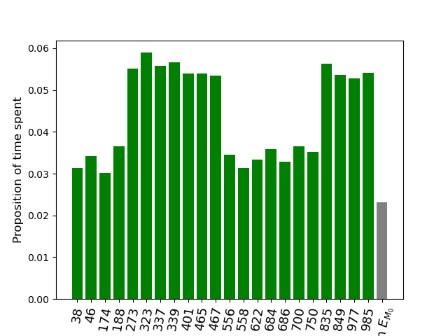
The following figure shows that the SEI-SLR algorithm covers properly the selection event without being stuck in one specific state of \(E_{M}\). The simulated annealing path is jumping from one state of \(E_{M}\) to another, ending up with an asymptotic distribution of the visited states that approximates the uniform distribution on \(E_{M}\).

model.histo_time_in_selection_event(states, ls_states_admissibles, rotation_angle=80)
plt.show()