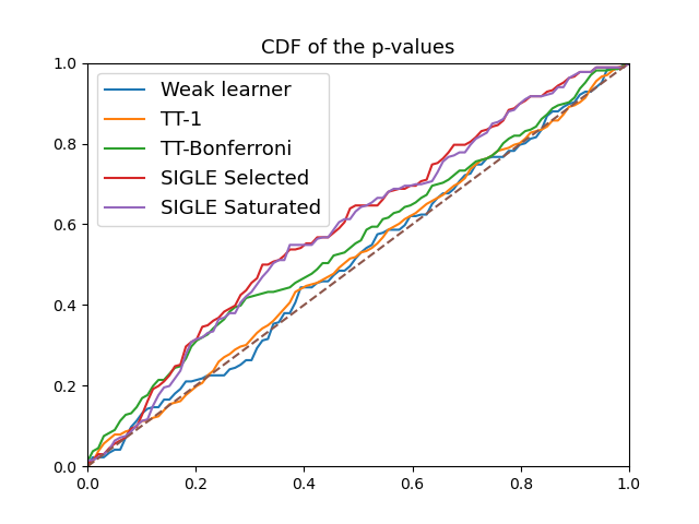
CDF of p-values

The example shows the cumulative disribution function (CDF) of the p-values of different post-selection inference methods for a composite hypothesis testing problem with a global null.

import PSILOGIT
import numpy as np
from PSILOGIT.tools import *
from sklearn.linear_model import LogisticRegression, LogisticRegressionCV
import matplotlib.pyplot as plt

Choice of the signal strength

nu = 0.1

Choice of the type of alternative (localized or disseminated)

modes = ['disseminated-signal' ,'localized-signal']
mode = modes[0]

Choice of the number of steps for the rejection sampling method

nb_ite = 100000

Definition of the experiment.

if mode=='localized-signal':
    vartheta = np.zeros(10)
    vartheta[0] = nu
else:
    vartheta = nu*np.ones(10)

model = PSILOGIT.PSILOGIT(truetheta=vartheta, regularization=2, n=100, p=10)
print('Size of the set of active variables: ', len(model.M))

Size of the set of active variables:  7

Sampling states according to the conditional distribution using the rejection sampling method.

states = model.SEI_by_sampling(model.sig, nb_ite=nb_ite)

0%|          | 0/100000 [00:00<?, ?it/s]

Sampling states according to the conditional distribution using the rejection sampling method under the global null.

thetanull = np.zeros(model.X.shape[1])
signull = sigmoid(model.X @ thetanull)
if np.max(np.abs(signull-model.sig))<1e-3:
    statesnull = np.copy(states)
else:
    statesnull = model.SEI_by_sampling(signull, nb_ite=nb_ite)

0%|          | 0/100000 [00:00<?, ?it/s]

p-values for the SIGLE procedures

tildeGN12, barpi = model.params_saturated(signull, statesnull)
lspvals_selec, lspvals_sat, gaps = model.pval_SIGLE(states, barpi, l2_regularization=100000, grad_descent={'lr':0.01,'return_gaps':True,'max_ite':10000}, calibrated_from_samples=True, statesnull=statesnull)

0%|          | 0/260 [00:00<?, ?it/s]
0%|          | 0/266 [00:00<?, ?it/s]
0%|          | 0/260 [00:00<?, ?it/s]

p-values for the procedures derived from the work of Taylor & Tibshirani

gamma = np.zeros(len(model.M))
gamma[0] = 1
lspvals_tay_1 = model.pval_taylor(states, thetanull=thetanull, gamma=gamma)
lspvals_tay_Bon = model.pval_taylor(states, thetanull=thetanull, mode='Bonferroni')

0%|          | 0/266 [00:00<?, ?it/s]
0%|          | 0/266 [00:00<?, ?it/s]
0%|          | 0/266 [00:00<?, ?it/s]
0%|          | 0/266 [00:00<?, ?it/s]
0%|          | 0/266 [00:00<?, ?it/s]
0%|          | 0/266 [00:00<?, ?it/s]
0%|          | 0/266 [00:00<?, ?it/s]
0%|          | 0/266 [00:00<?, ?it/s]

p-values for the weak learner

lspvals_naive = model.pval_weak_learner(statesnull, states, barpi, signull=signull)

0%|          | 0/260 [00:00<?, ?it/s]
0%|          | 0/266 [00:00<?, ?it/s]

CDF of pvalues

lists_pvalues = [lspvals_naive, lspvals_tay_1, lspvals_tay_Bon, lspvals_selec, lspvals_sat]
names = ['Weak learner', "TT-1", 'TT-Bonferroni', 'SIGLE Selected', 'SIGLE Saturated']
model.plot_cdf_pvalues(lists_pvalues, names, states = states, sigalt=model.sig)
plt.show()